Quick Start
This tutorial provides a quick start to the Calzone package, including a discussion of the installation and the basic command line interface usage.
The Calzone package includes a variety of commonly used calibration metrics. Expected Calibration Error (ECE) summarizes the average difference between predicted probabilities and actual outcomes across bins. Maximum Calibration Error (MCE) reports the worst-case deviation among bins. Hosmer-Lemeshow (HL) statistic compares observed and expected frequencies across groups to detect lack of fit, often used in medical risk modeling. Integrated Calibration Index (ICI) measures the average
absolute difference between predicted probabilities and observed frequencies across the entire probability range using curve fitting. Spiegelhalter’s Z-statistic tests whether predicted probabilities are systematically too high or too low, based on a normal approximation. Cox’s calibration slope and intercept are obtained by regressing the log odds of predicted probabilities against the observed outcomes, where a slope of 1 and an intercept of 0 indicate perfect calibration. Many of these
metrics can be computed either for the top predicted class or for each class individually, with user-defined binning schemes.
Installation
We recommend that you install Calzone from pip:
[ ]:
pip install calzone-tool
Alternatively, you can install the package and its dependencies manually. Calzone has very few dependencies: NumPy, SciPy, Statsmodels and Matplotlib:
[ ]:
pip install numpy
pip install scipy
pip install matplotlib
pip install statsmodels
Then, the package can be installed directly from the GitHub repository:
[ ]:
pip install -e "git+https://github.com/DIDSR/calzone.git"
Note that if you wish to use the experimental GUI interface, you will also need the additional dependency NiceGUI (pip install nicegui).
Command line interface
First, you need to prepare your dataset in a specific format. The dataset should be a CSV file with the following columns:
proba_0, proba_1, …, proba_n, label
where n >= 1. The proba_i columns are the probabilities of the i-th class, and the label column is the true class label.
Or if you have subgroups, the dataset should be a CSV file with the following columns:
proba_0, proba_1, …, proba_n, subgroup_1, subgroup_2, …, subgroup_m, label
where n >= 1 and m >= 1. The subgroup_j columns are the values of the j-th subgroup type, and its values should be categorical.
In the case of multi-class, you need to specify the class-of-interest, and the problem will be treated as 1-vs-all binary classification. To test the full calibration of the whole model, you need to test the calibration of each class.
The program also works if your csv file has no header.It will assume the first [:-1] columns are the probabilities and the last column is the label.
We have provided example datasets in the examples folder to illustrate the CSV input format Calzone expects.
[6]:
### For illuration purpose , I will use the functions in the helper.py in the local directory
### The data is generated using beta-binomial distribution


from helper import * #import local helper functions for example data generation

generate_wellcal_data(5000,"../../../example_data/simulated_welldata.csv",alpha_val=0.5, beta_val=0.5,random_seed=123)
generate_miscal_data(5000,"../../../example_data/simulated_misdata.csv", miscal_scale=2,alpha_val=0.5, beta_val=0.5,random_seed=123)
generate_subgroup_data(5000,"../../../example_data/simulated_data_subgroup.csv",miscal_scale=2,alpha_val=0.5, beta_val=0.5,random_seed=123)
[3]:
### Snippet of the csv file format
#Without subgroups
import numpy as np
print("Without subgroups")
print(np.loadtxt('../../../example_data/simulated_welldata.csv',dtype=str)[:5]) #first 5 lines of the without subgroups csv files
#With subgroups
print("With subgroups")
print(np.loadtxt('../../../example_data/simulated_data_subgroup.csv',dtype=str)[:5]) #first 5 lines of the with subgroups csv files
Without subgroups
['proba_0,proba_1,label'
 '1.444156178040510996e-01,8.555843821959489004e-01,0.000000000000000000e+00'
 '8.552048445812980848e-01,1.447951554187018874e-01,0.000000000000000000e+00'
 '2.569696048872897043e-01,7.430303951127102957e-01,0.000000000000000000e+00'
 '3.993130565553012490e-01,6.006869434446987510e-01,1.000000000000000000e+00']
With subgroups
['proba_0,proba_1,subgroup_1,label'
 '0.1444156178040511,0.8555843821959489,A,0'
 '0.8552048445812981,0.1447951554187019,A,0'
 '0.2569696048872897,0.7430303951127103,A,0'
 '0.39931305655530125,0.6006869434446988,A,1']
To use the command line interface (CLI), you can use the script in the calzone directory. The program will save the metrics into the output csv file with the CI (if you turn on boostrap). The program will also save the relibaility diagram if you apply –plot flag. There is an optional flag –prevalence_adjustment which tries to derive the original model prevalence and apply prevalence adjustment. See more on prevalence adjustment in the prevalecne adjustment notebook.
[1]:
# Use -h to see the help message and options
%run ../../../cal_metrics.py -h
usage: cal_metrics.py [-h] [--csv_file CSV_FILE] [--metrics METRICS]
                      [--prevalence_adjustment] [--n_bootstrap N_BOOTSTRAP]
                      [--bootstrap_ci BOOTSTRAP_CI]
                      [--class_to_calculate CLASS_TO_CALCULATE]
                      [--num_bins NUM_BINS]
                      [--hl_test_validation HL_TEST_VALIDATION] [--topclass]
                      [--save_metrics SAVE_METRICS] [--plot]
                      [--plot_bins PLOT_BINS] [--save_plot SAVE_PLOT]
                      [--save_diagram_output SAVE_DIAGRAM_OUTPUT] [--verbose]

Calculate calibration metrics and visualize reliability diagram.

options:
  -h, --help            show this help message and exit
  --csv_file CSV_FILE   Path to the input CSV file. (If there is header,it
                        must be in: proba_0,proba_1,...,subgroup_1(optional),s
                        ubgroup_2(optional),...label. If no header, then the
                        columns must be in the order of
                        proba_0,proba_1,...,label)
  --metrics METRICS     Comma-separated list of specific metrics to calculate
                        (SpiegelhalterZ,ECE-H,MCE-H,HL-H,ECE-C,MCE-C,HL-
                        C,COX,Loess,all). Default: all
  --prevalence_adjustment
                        Perform prevalence adjustment (default: False)
  --n_bootstrap N_BOOTSTRAP
                        Number of bootstrap samples (default: 0)
  --bootstrap_ci BOOTSTRAP_CI
                        Bootstrap confidence interval (default: 0.95)
  --class_to_calculate CLASS_TO_CALCULATE
                        Class to calculate metrics for (default: 1)
  --num_bins NUM_BINS   Number of bins for ECE/MCE/HL calculations (default:
                        10)
  --hl_test_validation HL_TEST_VALIDATION
                        Using nbin instead of nbin-2 as HL test DOF. Use it if
                        the dataset is validation set.
  --topclass            Whether to transform the problem to top-class problem.
  --save_metrics SAVE_METRICS
                        Save the metrics to a csv file
  --plot                Plot reliability diagram (default: False)
  --plot_bins PLOT_BINS
                        Number of bins for reliability diagram
  --save_plot SAVE_PLOT
                        Save the plot to a file. Must end with valid image
                        formats.
  --save_diagram_output SAVE_DIAGRAM_OUTPUT
                        Save the reliability diagram output to a file
  --verbose             Print verbose output
[8]:
%run ../../../cal_metrics.py \
--csv_file '../../../example_data/simulated_welldata.csv' \
--metrics all \
--n_bootstrap 1000 \
--bootstrap_ci 0.95 \
--class_to_calculate 1 \
--num_bins 10 \
--save_metrics '../../../example_data/simulated_welldata_result.csv' \
--plot \
--plot_bins 10 \
--save_plot '../../../example_data/simulated_welldata_result.png' \
--verbose \
--save_diagram_output '../../../example_data/simulated_welldata_diagram_output.csv'
### save_diagram_output only when you want to save the reliability diagram output
#--prevalence_adjustment # only when you want to apply prevalence adjustment
#--hl_test_validation #use it only when the data is from validation set
Metrics with bootstrap confidence intervals:
SpiegelhalterZ score: 0.376 (-1.581, 2.396)
SpiegelhalterZ p-value: 0.707 (0.017, 0.971)
ECE-H topclass: 0.01 (0.006, 0.021)
ECE-H: 0.012 (0.011, 0.025)
MCE-H topclass: 0.039 (0.016, 0.076)
MCE-H: 0.048 (0.034, 0.107)
HL-H score: 8.885 (7.392, 34.058)
HL-H p-value: 0.352 (0.000, 0.495)
ECE-C topclass: 0.009 (0.007, 0.021)
ECE-C: 0.009 (0.008, 0.022)
MCE-C topclass: 0.021 (0.018, 0.072)
MCE-C: 0.023 (0.020, 0.071)
HL-C score: 3.695 (4.778, 28.666)
HL-C p-value: 0.884 (0.000, 0.781)
COX coef: 0.994 (0.940, 1.054)
COX intercept: -0.045 (-0.126, 0.031)
COX coef lowerci: 0.937 (0.886, 0.994)
COX coef upperci: 1.051 (0.994, 1.114)
COX intercept lowerci: -0.123 (-0.205, -0.049)
COX intercept upperci: 0.034 (-0.048, 0.109)
COX ICI: 0.006 (0.001, 0.016)
Loess ICI: 0.006 (0.004, 0.016)
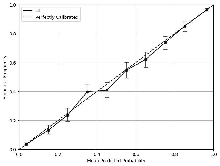
We use the CLI to compute the metrics and reliability diagram for the example dataset. The metrics and its 95% confidence interval will be printed and saved in a file. The reliability diagram will be saved in a separate file.
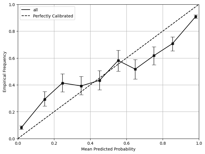
We can also test it on a miscalibrated dataset. The miscalibration is introduced by mutliply the log of probabilities by 2 and convert it back to probabilities.
[9]:
%run ../../../cal_metrics.py \
--csv_file '../../../example_data/simulated_misdata.csv' \
--metrics all \
--n_bootstrap 1000 \
--bootstrap_ci 0.95 \
--class_to_calculate 1 \
--num_bins 10 \
--save_metrics '../../../example_data/simulated_misdata_result.csv' \
--plot \
--plot_bins 10 \
--save_plot '../../../example_data/simulated_misdata_result.png' \
--verbose
Metrics with bootstrap confidence intervals:
SpiegelhalterZ score: 29.626 (26.37, 33.185)
SpiegelhalterZ p-value: 0. (0., 0.)
ECE-H topclass: 0.081 (0.073, 0.091)
ECE-H: 0.081 (0.073, 0.092)
MCE-H topclass: 0.151 (0.127, 0.202)
MCE-H: 0.168 (0.145, 0.244)
HL-H score: 1027.940 (818.524, 1292.977)
HL-H p-value: 0. (0., 0.)
ECE-C topclass: 0.079 (0.069, 0.09)
ECE-C: 0.08 (0.07, 0.091)
MCE-C topclass: 0.168 (0.141, 0.204)
MCE-C: 0.158 (0.139, 0.203)
HL-C score: 1857.584 (1355.637, 3341.319)
HL-C p-value: 0. (0., 0.)
COX coef: 0.497 (0.470, 0.524)
COX intercept: -0.045 (-0.125, 0.038)
COX coef lowerci: 0.469 (0.443, 0.494)
COX coef upperci: 0.526 (0.497, 0.554)
COX intercept lowerci: -0.123 (-0.203, -0.041)
COX intercept upperci: 0.034 (-0.046, 0.116)
COX ICI: 0.078 (0.071, 0.085)
Loess ICI: 0.074 (0.065, 0.083)
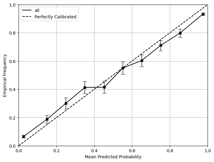
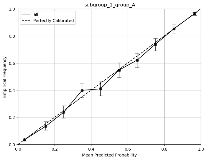
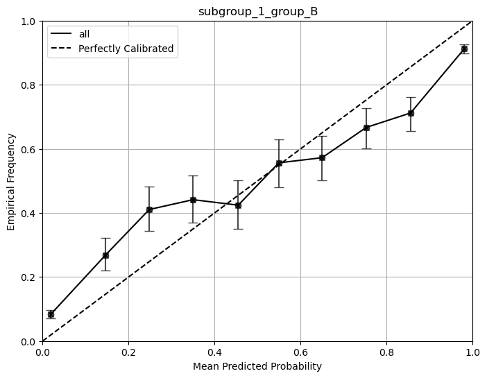
If your data has subgroups in it, simply run the script with the same argument as the one above. It will automatically detect the subgroup and generate the corresponding plots and metrics for each subgroup as well as the overall plot and metrics.
[10]:
%run ../../../cal_metrics.py \
--csv_file '../../../example_data/simulated_data_subgroup.csv' \
--metrics all \
--n_bootstrap 1000 \
--bootstrap_ci 0.95 \
--class_to_calculate 1 \
--num_bins 10 \
--save_metrics '../../../example_data/simulated_data_subgroup_result.csv' \
--plot \
--plot_bins 10 \
--save_plot '../../../example_data/simulated_data_subgroup_result.png' \
--verbose
Metrics with bootstrap confidence intervals:
SpiegelhalterZ score: 18.327 (15.794, 21.009)
SpiegelhalterZ p-value: 0. (0., 0.)
ECE-H topclass: 0.042 (0.035, 0.049)
ECE-H: 0.042 (0.036, 0.049)
MCE-H topclass: 0.055 (0.043, 0.087)
MCE-H: 0.063 (0.055, 0.109)
HL-H score: 429.732 (335.116, 584.729)
HL-H p-value: 0. (0., 0.)
ECE-C topclass: 0.042 (0.035, 0.049)
ECE-C: 0.038 (0.032, 0.046)
MCE-C topclass: 0.065 (0.055, 0.091)
MCE-C: 0.064 (0.052, 0.086)
HL-C score: 1138.842 (779.577, 1844.15)
HL-C p-value: 0. (0., 0.)
COX coef: 0.668 (0.638, 0.698)
COX intercept: -0.02 (-0.073, 0.03)
COX coef lowerci: 0.641 (0.611, 0.67)
COX coef upperci: 0.696 (0.664, 0.727)
COX intercept lowerci: -0.074 (-0.127, -0.025)
COX intercept upperci: 0.034 (-0.019, 0.084)
COX ICI: 0.049 (0.044, 0.055)
Loess ICI: 0.037 (0.032, 0.043)
Metrics for subgroup_1_group_A with bootstrap confidence intervals:
SpiegelhalterZ score: 0.376 (-1.536, 2.249)
SpiegelhalterZ p-value: 0.707 (0.018, 0.981)
ECE-H topclass: 0.01 (0.006, 0.021)
ECE-H: 0.012 (0.011, 0.025)
MCE-H topclass: 0.039 (0.017, 0.077)
MCE-H: 0.048 (0.034, 0.107)
HL-H score: 8.885 (7.273, 34.6)
HL-H p-value: 0.352 (0.000, 0.507)
ECE-C topclass: 0.009 (0.007, 0.022)
ECE-C: 0.009 (0.007, 0.023)
MCE-C topclass: 0.021 (0.018, 0.072)
MCE-C: 0.023 (0.018, 0.075)
HL-C score: 3.695 (4.463, 29.686)
HL-C p-value: 0.884 (0.000, 0.813)
COX coef: 0.994 (0.942, 1.050)
COX intercept: -0.045 (-0.135, 0.028)
COX coef lowerci: 0.937 (0.888, 0.990)
COX coef upperci: 1.051 (0.996, 1.111)
COX intercept lowerci: -0.123 (-0.214, -0.051)
COX intercept upperci: 0.034 (-0.056, 0.107)
COX ICI: 0.006 (0.001, 0.017)
Loess ICI: 0.006 (0.003, 0.016)
Metrics for subgroup_1_group_B with bootstrap confidence intervals:
SpiegelhalterZ score: 27.936 (24.631, 31.175)
SpiegelhalterZ p-value: 0. (0., 0.)
ECE-H topclass: 0.077 (0.068, 0.086)
ECE-H: 0.077 (0.069, 0.087)
MCE-H topclass: 0.133 (0.108, 0.175)
MCE-H: 0.163 (0.13, 0.232)
HL-H score: 910.439 (716.681, 1156.971)
HL-H p-value: 0. (0., 0.)
ECE-C topclass: 0.074 (0.066, 0.084)
ECE-C: 0.075 (0.065, 0.085)
MCE-C topclass: 0.141 (0.124, 0.182)
MCE-C: 0.140 (0.115, 0.182)
HL-C score: 2246.171 (1393.175, 3900.391)
HL-C p-value: 0. (0., 0.)
COX coef: 0.507 (0.481, 0.539)
COX intercept: 0.000 (-0.073, 0.077)
COX coef lowerci: 0.478 (0.454, 0.508)
COX coef upperci: 0.536 (0.508, 0.569)
COX intercept lowerci: -0.078 (-0.152, -0.002)
COX intercept upperci: 0.079 (0.005, 0.155)
COX ICI: 0.077 (0.07, 0.085)
Loess ICI: 0.07 (0.062, 0.078)
Using Calzone in python
Instead of running the command line tool, you can also use Calzone in python directly
[1]:
from calzone.metrics import CalibrationMetrics
from calzone.utils import data_loader

loader = data_loader('../../../example_data/simulated_welldata.csv')
cal_metrics = CalibrationMetrics(class_to_calculate=1)
cal_metrics.calculate_metrics(loader.labels, loader.probs, metrics='all')
[1]:
{'SpiegelhalterZ score': 0.3763269161877356,
 'SpiegelhalterZ p-value': 0.7066738713391099,
 'ECE-H topclass': 0.009608653731328977,
 'ECE-H': 0.01208775955804901,
 'MCE-H topclass': 0.03926468843081976,
 'MCE-H': 0.04848338618970194,
 'HL-H score': 8.884991559088098,
 'HL-H p-value': 0.35209071874348785,
 'ECE-C topclass': 0.009458033653818828,
 'ECE-C': 0.008733966945443138,
 'MCE-C topclass': 0.020515047600205505,
 'MCE-C': 0.02324031223486256,
 'HL-C score': 3.694947603203135,
 'HL-C p-value': 0.8835446575708198,
 'COX coef': 0.9942499557748269,
 'COX intercept': -0.04497652296600376,
 'COX coef lowerci': 0.9372902801721911,
 'COX coef upperci': 1.0512096313774626,
 'COX intercept lowerci': -0.12348577118577644,
 'COX intercept upperci': 0.03353272525376893,
 'COX ICI': 0.005610391483826338,
 'Loess ICI': 0.00558856942568957}